Given a data path $DP(M_o\cup M_s \cup M_i,I)$ , a scheduled DFG $G(V_o\cup V_s,E,C)$ and a module library $\Lambda(T,L)$ :

Module allocation: the module allocation function $\mu :V_o\rightarrow \Pi(M_o)$ , determines which module performs a given operation.

Note that a module allocation $\mu(v_i)=m, m\in M_o, v_i\in V_o$ can only be a valid allocation if $m\in \lambda(\tau (v_i))$ , i.e. the module $m$ is capable of execution of operation type of $v_i$ .

Module binding: a resource binding is a mapping $\beta : V_o\rightarrow M_o \times N$ , where $\beta(v_o) = (t,r)$ denotes that the operation corresponding to $v_o \in V_o$ , with type $\tau(v_o)\in \lambda^{-1}(t)$ (i.e. component $t\in L$ can execute the operation represented by vertex $v_o$ ), is executed on the component $t = \mu(v_o)$ and $r< \sigma(t)$ (i.e. the operation is implemented by the r-th instance of resource type $t$ and this instance is available into datapath).

A simple case of binding is a dedicated resource. Each operation is bound to one resource, and the resource binding $\beta$ is a one-to-one function.

A resource binding may associate one instance of a resource type to more than one operation. In this case, that particular resource is shared and binding is a many-to-one function. A necessary condition for a resource binding to produce a valid circuit implementation is that the operations corresponding to a shared resource do not execute concurrently, i.e. they are in mutual exclusion.

When binding constraints are specified, a resource binding must be compatible with them. In particular, a partial binding may be part of the original specification, as described in Binding constraints. This corresponds to specifying a binding for a subset of the operations $U\subseteq V_o$ . A resource binding is compatible with a partial binding when its restriction to the operations $U$ is identical to the partial binding itself.

Introduction

The module allocation is one of subproblems which high level synthesis problem is decomposed in. Here you focus on assignement of modules to all operations into data path.

First, it's fundamental to give some general definition about module allocation problem and then analyse this and corresponding algorithms implemented.

Module allocation problem definition

Given a data path DP $(M_o\cup M_s\cup M_i,I)$ , a scheduled DFG $G(V_o\cup V_s,E,C)$ and a module library $\Lambda (T,L)$ :

The module allocation function: $\mu :V_o \rightarrow \Pi (M_o)$ determines which module performs a given operation.

Note that a module allocation $\mu (v_i)=m, m\in M_o, v_i\in V_o$ can only be a valid allocation if $m\in \lambda (\tau (v_i)),$ i.e. the module m is capable of execution the operation type of $v_i$ .

Compatibility graph definition

Module allocation problem can be modeled using a module allocation graph. A compatibility graph $G_o(V_o,Y)$ is defined where:

$Y={ \lbrace (v_i,v_j)\mid (\theta (v_i)\cap \theta (v_j)=\emptyset )\vee (m(v_i) \wedge m(v_j)=[0])\wedge \lambda (\tau (v_i)) \cap \lambda (\tau (v_j)) \neq \emptyset \rbrace }$

An edge $y\in Y$ is added between two nodes if the two operations they represents can be combined in a single module, i.e. the operations do not have to be executed concurrently (they are scheduled into different steps) or are mutually exclusive and there exists a module that can perform both operations.

Despite the fact that the register allocation and module allocation look fairy similar there are some differences. In the register allocation it was quietly assumed that all values could be merged in a register. This may not be the case if registers of different bitwidth are considered. But even in this case the transitivity property remains. If value a and b can be fit into a register and so do b and c, also a and c will fit since there has to be a register of size at least the maximum width of a, b and c. In module allocation this is not necessary the case. certain restrictions are imposed on the schedule, module allocation can become considerable simpler. If the schedule does not contain operations that are scheduled over multiple cycle steps (multicycling), this will be called a simple schedule. A data flow graph that does not contain conditional branches will be called an unconditional data flow graph.

Library definitions and properties

First, some library definitions and proprieties on high level synthesies problem can be given.
The data flow graph (graph_manager::DFG) describes the input design to a high level synthesis system. A system needs also information on which modules can be used during the synthesis. A collection of these modules are represented by a library. It is common to use a set of modules each of which can only execute a limited set of operations. The library provides a way to describe the relation between the types of operations and the modules.

The library $\Lambda (T,L)$ is definited by a set of operation types T and the set of components L. The library function $\lambda : T \rightarrow \Pi (L)$ , determines for each operation type $t \in T$ by which components it can be performed. So the function $\lambda ^ {-1}: L \rightarrow \Pi (T)$ describes for each component which types of operations it can execute. The set $\lambda ^ {-1}(i)$ will be called operation type set of l. Operations whose type belong to the same operation type set can share a module (there is a module that can perform both).

The operation type set function $\Omega : L \rightarrow \Pi (O)$ , gives for each library component $l \in L$ , which operation types it can execute. The sets $\Omega (l),l \in L$ will be called the operation type sets of the library $\lambda (O,L)$ .

A library $\Lambda (O,L)$ is called a ordered library, if the operation type sets of $\Lambda (O,L)$ form a partial ordering by the set inclusion relation, where all maximal sets are disjunct, which means that all the maximal sets have not a operation type that can be performed by two different maximal components.

An ordered set can be depicted conveniently by a Hasse diagram (performed in technology_manager::check_library), in which each element is represented by a point, so placed that if $X \subset Y$ , the point representing X lies below the point representing Y. Lines are drawn to connect sets of X and Y such that Y covers X, i.e. $X \subset Y$ and there is not set Z such that $X \subset Z \subset Y$ ; this is implemented by a directed (covering) edge in a look-like Hasse diagram. A subset is maximal if it's not covered by any other and so it's maximal if it hasn't any incoming edge.

A library is called complete if the library is ordered and has only one maximal set.

A library is called ordered with respect to a DFG, if all the operation types in DFG are an element of one of the maximal operation type sets. Similary, a library is called complete with respect to a DFG, if the maximal operation type set (it's only one) contains all operation types in the DFG. In the remainder of this description the terms complete and ordered libreries will always be used with respect to a DFG.

Impact of libraries on compatibility graphs: comparability graphs

Now, how a library can impact on module allocation graphs should be analysed.

First, it could be useful to remember most important properties of comparability graphs.
An undirected graph $G(V,E)$ is called a comparability graph if each edge can be assigned a one way direction, in such a way that the resulting oriented graph $G(V,T)$ satisfies the following condition:

$[v_i,v_j]\in T \wedge [v_j,v_k]\in T \Rightarrow [v_i,v_k]\in T$ $\forall v_i,v_j,v_k \in V$

Comparability graphs are often called transitivity orientable graphs. A relation is called a partial ordering of a set A, when it is reflexive, anti-symmetric and transitive. The relation T is a partial ordering defined on a set V, called the transitive orientation of G.

A module allocation graph derived from an unconditional DFG with a simple schedule and a complete library is a comparability graph (and so it's transitive and orientable).

A module allocation graph derived from and unconditional DFG with a simple schedule and an ordered library is a comparability graph.
Since the library is ordered the composition will result in a module allocation graph consisting of m disjoint comparability graphs, where m is the number of maximal operation types sets in the library of which elements are present in the data flow graphs. In fact flow_allocation can be applied to separated flow network, one for each operation type sets (module_binding::net_flow, passing operation type as a parameter)

A module allocation graphs derived from a DFG with a schedule with property the when operations from a branch are scheduled in the same cycle steps with operations from at most one of its successors branches, and an ordered library, is a comparability graphs.
That's why in module_binding::create_graph has been performed a check is DFG contains or not only nested conditional operations; in fact, these algorithms can operate also with conditional operations, only if there are not nested.

Weighted module allocation

We start from a schedule applied before and then operations are been pre-allocated by algorithms choosen before. The result is a sequence of scheduled operations, with an initial allocation to operation type sets representing functional units that are in technology library.
Module allocation in isolation deals with minimizing the number of operational modules. Now the problem is to improve this module allocation with algorithms exploiting some operation proprieties or considering other aspects of data path allocation. Examples are cost modules or their interconnections. For example, operations can be combined with similar inputs and outputs to reduce the interconnections. Source and destinations of values therefore have to be known. If Register allocation has been performed most inputs and outputs values to the operations are known. So operations can be relocated if results are stored in (or inputs come from) same registers and put in the same functional unit module: this has been implemented in module_binding::weighted_allocation (an algorithm based on progressive thresholds) and module_binding::flow_allocation (flow networks to resolve module allocation problem) with different algorithms.
To model preferences in sharing of operations, weight categories can be assigned to edges in the comparability graph. The edge weight is a measure for the number of common inputs and outputs two operations have (performed in module_binding::create_graph while it's going to create graph). Since the operation nodes are not yet allocated, only the inputs and outputs that have the same operation as origin and destination can be counted. That's been implemented in two different version of module_binding::get_reg_op, one for inputs (reading GET_VAR_READ list) and one for outputs (reading GET_VAR_WRITTEN list).

an algorithm based on progressive thresholds

An heuristic algorithm can be used to find the cliques in a weighted graph. The heuristic presented in module_binding::minimal_clique can be extended. Let $G_{th}(V_{o},Y,W)$ be a graph induced by the edges with weight larger than or equal to the threshold value th. A clique covering is done on this $G_{th}$ . Vertices which form a clique in $G_{th}$ will be combined in G. Appropriate edges are removed and the weights are update. A new graph is induced with a lower value for the threshold. This process iterates until no new cliques are found and the threshold is low enough to include all remaining edges.
This algorithm has been implemented in module_binding::clique_cover as follow
The allocation graph is $ G(V,E)$ (where V is set of clique-vertices and E is set of edges) and $ C(T,R)$ is comparability graph (where T is his set of operation-vertices and R is his set of edges):

$\\.find\_maximum\_threshold(C); \\ .\mathbf{foreach}\ op \in T\ \ \mathbf{do} \\ .\ \ \ \ \ v=\lbrace op \rbrace \ \ \textrm{ / / create a vertex-clique with only operation op } \\ .\ \ \ \ \ V=V \cup \lbrace v \rbrace\ \\ .\mathbf{endfor}\\ .\mathbf{foreach}\ ed \in R\ \ \mathbf{do} \\ .\ \ \ \ \ e=\lbrace (s,t)\ \mid s=\lbrace source(ed) \rbrace\ \ \wedge\ \ t=\lbrace target(ed) \rbrace \rbrace\ \ \textrm{ / / populate E } \\ .\ \ \ \ \ E=E \cup \lbrace e \rbrace\ \\ .\mathbf{endfor}\\ .\mathbf{repeat}\\ .\ \ \ \ \ G_{th}=G; \\ .\ \ \ \ \ th=compute\_max\_threshold(G_{th}); \\ .\ \ \ \ \ \mathbf{foreach}\ \ e \in E_{th}\ \ \mathbf{do} \\ .\ \ \ \ \ \ \ \ \ \ \mathbf{if}\ \ weight(e) < th\ \ \mathbf{then} \\ .\ \ \ \ \ \ \ \ \ \ \ \ \ \ \ E_{th} = E_{th} \setminus e \\ .\ \ \ \ \ \ \ \ \ \ \mathbf{endif} \\ .\ \ \ \ \ \mathbf{endfor}\\ .\ \ \ \ \ \ L=compute\_clique\_cover\_on\_G_{th}\ \ \textrm{ / / create a list of clique } \\ .\ \ \ \ \ \mathbf{foreach}\ \ l \in L\ \ \mathbf{do} \\ .\ \ \ \ \ \ \ \ \ \ \ \ n = \emptyset \\ .\ \ \ \ \ \ \ \ \ \ \ \mathbf{foreach}\ \ v \in l\ \ \mathbf{do} \\ .\ \ \ \ \ \ \ \ \ \ \ \ \ \ \ \ \ G=G \setminus \lbrace v \rbrace \\ .\ \ \ \ \ \ \ \ \ \ \ \ \ \ \ \ \ n=n \cup \lbrace v \rbrace \\ .\ \ \ \ \ \ \ \ \ \ \ \mathbf{endfor}\\ .\ \ \ \ \ \ \ \ \ \ \ \ G = G \cup \lbrace n \rbrace \\ .\ \ \ \ \ \ \ \ \ \ \ \ update\_edges\_and\_weights(E) \ \ \textrm{ / / collapse vertices in G graph in a unique clique and update edges } \\ .\ \ \ \ \ \mathbf{endfor}\\ .\mathbf{until}\ \ th>1$
See Example and corresponding resolution with threshold algorithm

This heuristic will give no guarantee for optimality of the results. In the case of comparability graphs another technique can be employed.

flow networks to resolve module allocation problem

Comparability graphs are per definition transitively orientable. If a path $\langle \ a,b,c\ \rangle$ exists, the edge $ (a,c) $ is guaranteed to exist as well. Each path in the graph will therefore be a clique. So the reminder of this section will describe how to transform the weighted module allocation problem to network flow problem. The transformation to the network flow is a transformation generally valid for comparability graphs. It can therefore be used in the other allocation phases as well.

Consider the weighted module allocation graph $G_{o}(V_{o},T,W)$ . Furthermore, a source node a, a sink node z, edges from source node to all nodes, edges from all nodes to the sink node and an edge from the sink to the source are added. The edge from the sink to the source is called the return edge, The weight of all these additional edges is zero.
Formally, a network $N_{G}=(V_n,E_n,a,z,C,K)$ corresponding to the module allocation graph is constructed, where:

$V_n=V_o \cup \lbrace a,z \rbrace$ .
$E_n=T \cup \lbrace [a,v],[v,z] \mid v \in V_o \rbrace \cup \lbrace [z,a] \rbrace$ .
$w(a,v)=w(v,z)=0\ \ \forall v \in V_o,\ \ \ \ \ \ \ \ \ w(z,a)=0$ .

For each edge $e \in E_n$ a cost function $C: E_n \rightarrow \aleph$ is defined, which assigns to each edge a non-negative integer. The cost will be equal to the weight of the edges: $ C([u,v])=w(u,c) $ for all $[u,v] \in E_n$ .
For each edge $e \in E_n$ a capacity function $K:E_n \rightarrow \aleph$ is defined, which assigns to each edge a non-negative integer. The capacity of all edges is one, except for the return edge which has capacity k: $K([z,a])=k, \ \ \ \ \ \ \ \ \ \ \ K([u,v])=1 \ \ \ \ \forall [u,v] \in E_n \setminus \lbrace [z,a] \rbrace$ .

A flow in the network $ N_G $ is a function $f:E_n \rightarrow \aleph ^{+}$ , which assigns to each edge a non-negative integer, such that for $e \in E_n,O \leq f(e) \leq K(e)$ and for any node $u \in V_n$
$\sum _{[u,v]\in E_n} f(u,v) - \sum _{[v,u]\in E_n} f(v,u) \ \ \ \ \ \ \ \ \ \ \ \ \ \ \ \ \$ balancing equation

The amount of flow in the return edge $ [z,a] $ is denoted as $ F=f([z,a]) $ . The total cost of the flow is: $k(F)=\Sigma _{e\in E_n} C(e) \cdot f(e)$ .

A flow $f:E_n \rightarrow \aleph$ , in the network $ N_G $ corresponds to a set of cliques $ X_1,...,X_k $ in G_o where $ k=F $ .

The paths $ P_1,...,P_k $ will be edge disjoint (each edge has only capacity=1), but not necessarily go through different nodes (in a node can enter/exit more than one edge). Thus the sets are not necessarily node disjoint (a node can be in different cliques, so can be allocated into different modules).
To enforce node disjoint paths, a node separation technique can be used. In the node separation, all nodes $v \in V_o$ are duplicated. The duplicate of a node $ v $ is called $ v' $ . All edges outgoing from $ v $ , obtain the node $ v' $ as their origin. The node $ v $ and its duplicate are connected by an edge with capacity $ K([v,v'])=1 $ (only one unit flow can go through) and a cost $ C([v,v'])=0 $ (no additional solution cost). This node separation results in a network $ N'_G=(V'_n,E'_n,a,z,C',K') $ , where:

$V'_n=V_n \cup V'_o$
$\exists v',v'\in V'_o$ for each vertex $v \in V_o$
$E'_n=T \cup \lbrace [a,v],[v',z] \mid v \in V_o \rbrace \ \ \cup \ \ \lbrace [z,a] \rbrace \cup \lbrace [v,v']\mid v\in V_o \rbrace$
$T' = \lbrace [v',u]\mid [v,u] \in T\rbrace$
$C'([z,a])=C'([v,v']) = 0 \ \ \ \ \ \forall v \in V_o \ \ \ \$ (no additional cost for support edges)
$C'([v',u])=C([v,u]) \ \ \ \ \forall [v,v'] \in T' \cup \lbrace [a,v],[v',z]\mid v \in V_o$
$K'([z,a])=k \ \ \ \ \ \ \ \ \ K'([u,v])=1 \ \ \ \ \ \ \forall u \neq z \wedge v \neq a$

Since the capacity of $ K([v,v'])=1 $ at most one unit of flow can go through the edge [v,v']. This leads to the following theorem:

A flow $f:E'_n \rightarrow \aleph$ , in the network $ N'_G $ corresponds to a set of node disjoint cliques $ X_1,...,X_k $ in $ G_o $ where $ k=F $ .

The maximal cost network flow problem finds among all possible flows with amount k the one with maximum cost. This has been implemented in module_binding::maxcost_minflow function, where you can find a way to resolve maxcost flow with a positive cycles elimination. In fact, whenever you can find a positive cycle in the residual network flow, the solution can be incremented over this one and the new solution will be always better. So, if no positive cycles can be found, a better the solution cannot be found and the flow obtained is the maxcost one.

In this situation, a triple $ (G,s,l) $ is given where $ G=(V,E) $ is a directed graph with n vertices and m edges, $l:E \rightarrow R$ is a lenght function mapping edges to integer lenghts and $s \in V$ in the root vertex. The lenght of the path $\rho = \langle v_0,v_1,...,v_k \rangle$ is the sum of lenghts of its constituent edges (take it negative if the edge is a flow edge due to residual definition graph). So positive cycle is a cycle $\rho = \langle v_0,v_1,...,v_k,v_o \rangle$ with lenght $l(\rho )>0$ . Algorithms for PCD (positive cycle detection) that use the adjacency-list representation of the graph construct a longest-path tree $ G_s=(V_s,E_s) $ , where $ V_s $ is the set of all vertices reachable from the root s, $E_s \subseteq E$ , s is the root of $ G_s $ and for every vertex $v \in V_s$ the path from s to v in $ G_s $ is a longest path from s to v in G.
The labeling method maintains for every vertex v its distance label $ d(v) $ and parent $ p(v) $ . Initially $ d(v)=0 $ and $ p(v)=root $ . The method is based on the scan operation. During scanning a vertex v, all edges $ (v,u) $ out-going from v are relaxed which means that if $ d(u) < d(v) + l(v,u) $ then $ d(u) $ is set to $ d(v)+l(v,u) $ and $ p(u) $ is set to v. If all vertices have been scanned then d gives the longest path lenghts and $ G_p $ (parent graph induced by edges $ (p(v),v) $ ) is the longest path tree. So, if there is a cycle, after a finite number of scan operations ( $\mid V_g \mid$ is upper bound) you can detect it; in fact, starting from a vertex $ v_o $ , if the same vertex $ v_o $ is in parent tree, it means that there is a (positive) path from $ v_o $ to $ v_o $ , so there is a cycle.
Once detected a positive cycle, the flow on positive edges is increased and the flow on negative ones is decremented. So cycle is eliminated and solution cost will be better. If any positive cycle can be detected, there is no way to improve solution and this will be the best one (maximum cost solution).

See Example and corresponding resolution with flow network

When the maximal cost network flow is solved for the network $ N'_G $ , a solution to the module allocation problem is found, which takes into account the first order effects of interconnection weights. These first order effects describe the result of combining each pair of operations. Taking into account the influence of this combination on the weights with a third operation, would require a dynamic update of the edge weights due to the cumulative nature of the costs. This aspect has not been implemeted yet in this project.

Example

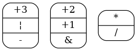
For example, having this DFG:

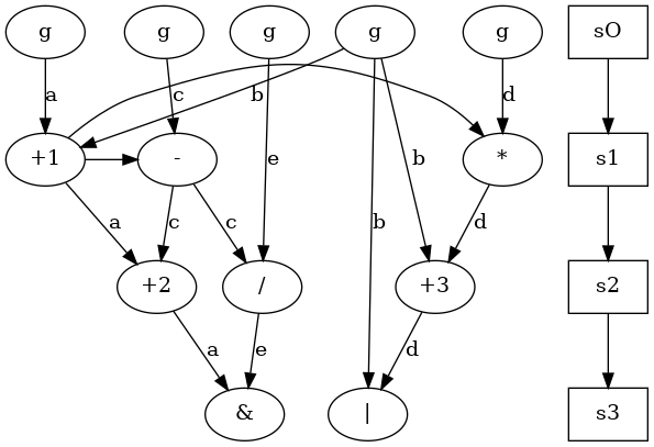
where egde label is register name where variable is stored and g are inputs.
Assuming a library with two functional unit types, one that can implement $\lbrace +,-,\&,\mid \rbrace$ and the other that implements $\lbrace *,/ \rbrace$ , comparability graph has to be created, according to definition given above (they are scheduled into different steps or they are in exclusive paths, they can be executed by same functional unit type).

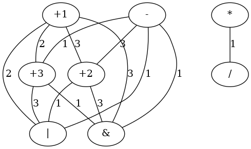
Edge label is weight value: number of commun inputs and outputs. For example, edge $ ('+1','+3') $ has $ w(e)=2 $ . In fact, assuming $ w(e)=1 $ as base, that means only one common input or output: that is register $ b $ that is a common input: both read from this one. Edge $ ('+1','+2') $ has a common input (they read both from register $ a $ ) and a common output (they write both to register $ a $ ); so it has $ w(e)=3 $ . Now, cliques have to be found in this (weighted) graph. It's important to notice that to do this a schedule and an assignement to functional units types have to be provided. These are provided by HLS class.

resolution with threshold algorithm

On the example above, threshold algorithm can be applied as described.
First maximum threshold is $ th=3 $ and so graph induced is:

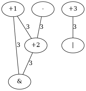
where, applying clique covering, three clique can be found: $\lbrace +1,+2,\& \rbrace$ , $\lbrace +3,| \rbrace$ and $\lbrace - \rbrace$ . So the comparability graph modified collapsing nodes and updating egdes (an edge remains if there was an edge beetween the node and each node in the new clique) is:

Now the choose to compute maximum threshold is shown to be efficent. In fact, there is not any edge $ w(e)=2 $ so the computation is applied with $ th=1 $ . The graph induced is the same (no edge is eliminated):

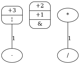
and two new clique are found: $\lbrace \lbrace +3, | \rbrace , - \rbrace$ and $\lbrace *,/ \rbrace$ . So, the new (and final) comparability graph is:

No edge is left and so vertices are definitive cliques. Each clique can be assigned to a module. So, operations with weighter edges are prefered to be assigned to same module.

resolution with flow network

On example above, there is not any nested conditional operation and so the compatility graph is orientable (it becomes a comparability graph). Thus a flow network for each FU type can be created as well. In according to definition given in subsection flow networks to resolve module allocation problem, the flow network for FU type $\lbrace +,-,\&,\mid \rbrace$ for resulting is:

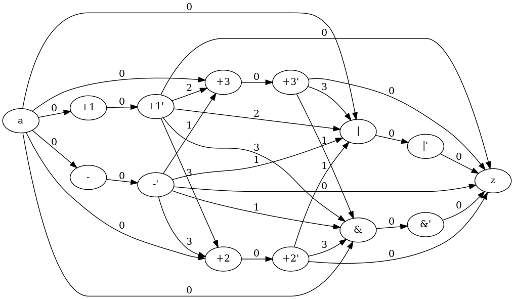
A dummy initial flow can be applied and corresponding residual graph will be:

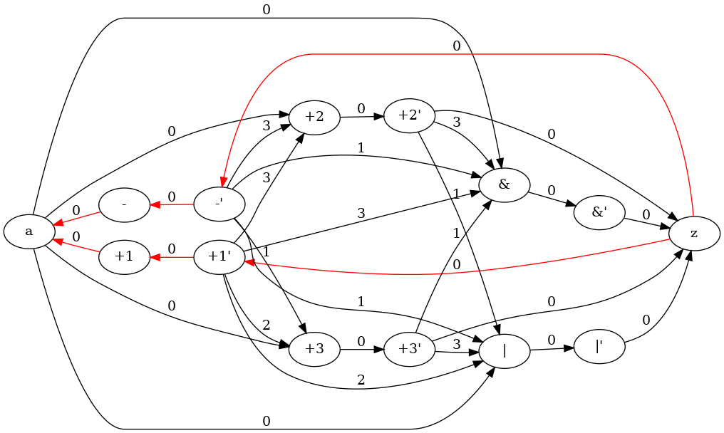
In this way, it's simple to find a better solution. When a positive cycle has been found (for example $\rho= <-',+2,+2',z,-'>$ and $l(\rho )=3)$ , the flow can be increased on direct edge and decreased in return edge. Thus solution would be better (from $ C=0 $ to $ C=3 $ ):

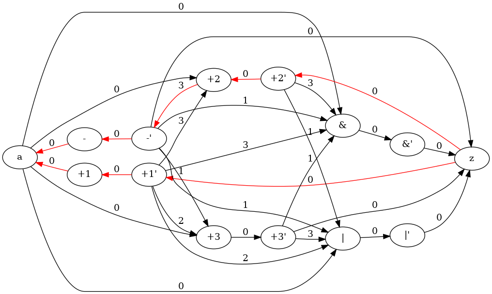
When no more positive cycles can be found, the solution is optimal for this network and the paths from source to sink will be the max cost partitioning for operation vertices present in this graph. This algorithm have to be applied to all functional units type the library consists in.